Preface
To understand the mathematical notations in this document, you may want to have a look at the summary of mathematical notations and conventions before reading on.
Introduction
The Quantum Spin Visualizer is an interactive application, which visualizes the spin state of quantum objects. It can visualize different types of objects, including spin 1 objects like photons and spin 1/2 objects like electrons.
Technically, a spin state is represented as a multi-dimensional array of complex numbers, in the simplest case as a two-dimensional array. These arrays are then visualized as 2D images, where the individual complex numbers correspond to the pixels of the image. The phase angle of a complex number is encoded as the pixel color, and the magnitude of the complex number is encoded as color intensity.
These visualizations are very helpful to understand the spin of quantum objects, because they mirror many mathematical properties of spin states, in particular:
- They visualize measurable properties of spin states like the polarization direction of photons or the spin direction of electrons.
- They can be phase-shifted and superimposed to create new spin states.
- They visualize the intrinsic angular momentum of certain spin states as a color gradient.
Feature Overview
The application not only visualizes a single spin state. Instead, it visualizes the process to construct a particular spin state by superimposing scaled and phase-shifted basis states according to the following formula:
\[ {\ \color{blue} \ket{\psi}} = a_1 {\ \color{blue} \ket{B_1}} + a_2 {\ \color{blue} \ket{B_2}} \]
Here \({\ \color{blue} \ket{B_1}}\) and \({\ \color{blue} \ket{B_2}}\) are basis states which are scaled and phase-shifted by the complex numbers \(a_1\) and \(a_2\) respectively, and then superimposed to get the result state \({\ \color{blue} \ket{\psi}}\). In the case of a two-level quantum system, you can get all possible system states by choosing the appropriate values for \(a_1\) and \(a_2\).
The application visualizes all of the following states: The basis states \({\ \color{blue} \ket{B_1}}\) and \({\ \color{blue} \ket{B_2}}\), the intermediate states \(a_1 {\ \color{blue} \ket{B_1}}\) and \(a_2 {\ \color{blue} \ket{B_2}}\), and the result state \({\ \color{blue} \ket{\psi}}\). In addition, it also visualizes the values of the complex numbers \(a_1\) and \(a_2\).
The user interface is organized as a grid, which has five distinct rows:
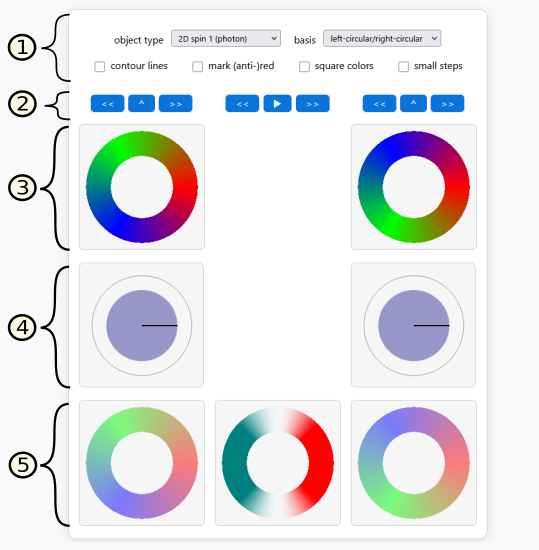
Row 1 contains configuration controls, which let you select the object type to be visualized, the basis states to use, and some display and animation options. See Section configuration controls for details.
Row 2 contains buttons to manipulate the amplitudes \(a_1\) and \(a_2\), which are visualized in row 4. See Section Buttons to Manipulate the Amplitudes for details.
Row 3 contains the visualizations of the basis states \({\ \color{blue} \ket{B_1}}\) and \({\ \color{blue} \ket{B_2}}\).
Row 4 contains the visualization of the complex numbers \(a_1\) and \(a_2\).
Row 5 contains the visualizations of the scaled basis states \(a_1 {\ \color{blue} \ket{B_1}}\) and \(a_2 {\ \color{blue} \ket{B_2}}\), as well as the result state \({\ \color{blue} \ket{\psi}}\).
Configuration Controls
The configuration controls in Row 1 are used to configure the following properties:
object type: Selects the physical/mathematical model that is visualized. The available options are:
2D spin 1 (photon)2D spin 1/2 v1 (neutrino?)2D spin 1/2 v2 (neutrino?)3D spin 1/2 (electron)
basis: Selects the pair of basis states \({\ \color{blue} \ket{B_1}}\) and \({\ \color{blue} \ket{B_2}}\) used for the superposition. Depending on the selected object type, different basis pairs are available, for example
horizontal/verticalfor photons orup/downfor electrons.contour lines: This option highlights pixels whose phase angle is a multiple of 22.5°. In other words: If the visualization contains a linear phase gradient from 0° to 360°, this option activates 16 equidistant contour lines.
mark (anti-)red: This option marks pixels whose phase angle is 0° (red) or 180° (anti-red). This can help to better see the overall orientation of the spin state.
square colors: This option applies a phase-doubling to the state visualization. This is helpful to explain spin 1/2 representations and their relation to 1 representations.
small steps: This option reduces the step size of button operations. This is useful for fine-grained adjustments of amplitudes and phase angles.
There is one hidden feature: If you press the keyboard button
X, an additional drop-down field “visualization” is shown.
It can be used to visualize the individual array layers of 3D spin 1/2
representations. For details, see section State Representation and
Visualization.
Buttons to Manipulate the Amplitudes
The buttons in Row 2 are used to manipulate the amplitudes in row 4.
The buttons in the left/right columns control the left/right amplitudes as follows:
<<rotates the phase angle of the corresponding amplitude counterclockwise.>>rotates the phase angle of the corresponding amplitude clockwise.^increases the scale factor of the corresponding amplitude, while simultaneously decreasing the scale factor of the other one, maintaining the normalization of scale factors.
The buttons in the middle column affect both the left and the right amplitude:
<<rotates the phase angle of both amplitudes counterclockwise.▶/⏸toggles between play/pause mode. In play mode the phase angles of both amplitudes are automatically rotated clockwise.
>>rotates the phase angle of both amplitudes clockwise.
By default, the step widths of the buttons are as follows:
- Phase rotation buttons: 1/32 of a full circle (i.e. a rotation of 11.25°)
- Scale factor buttons: 1/8 of a complete weight transfer
By activating the check box small steps, the step widths are divided by two.
There is one hidden feature: If you press one of the phase rotation buttons for individual amplitudes while holding the shift key, the other phase will be rotated in the opposite direction. This is helpful to rotate a 3D spinor state.
State Representation and Visualization
Each state (basis state, scaled basis state, and result state) is internally represented as a complex-valued array. In case of the 2D object types, a 200x200 array is used. In case of the 3D spinor type, a 200x200x2 array is used.
Visualization of a 200x200 array: A 200x200 array is visualized by converting each complex number into a color. The state is then visualized as an image with 200x200 pixels with the corresponding colors.
Each complex number is mapped to a color as follows:
- The phase angle is mapped to the color hue. 0° is mapped to red, 120° is mapped to green, 240° is mapped to blue, and intermediate phase angles are mapped to interpolated colors.
- The absolute value is mapped to color intensity/transparency. The value 1 (maximal value) is mapped to a completely opaque color, and the value 0 is mapped to a completely transparent color, i.e. you see the white background.
Visualization of a 200x200x2 array: In this case, the last dimension encodes a local spinor structure. By default, a local spinor structure with components \((c_1, c_2)\) is mapped to a color as follows: First, the complex value \(\pm \sqrt{c_1 c_2}\) is computed. Then this value is mapped to a color like in the 200x200 array case.
You can switch to a different visualization, which shows one of the
individual spinor structure layers, as follows. Press X on
the keyboard and then choose layer 1 or
layer 2 in the appearing drop-down field “visualization”.
If you choose layer 1, the \(c_1\) values are visualized as colors. If
you choose layer 2, the \(c_2\) values are visualized as colors.
Adding and scaling state vectors: The operations to add and scale complex-valued arrays are straightforward:
- To add two complex-valued arrays, the individual values are added pointwise.
- To scale a complex-valued array with a complex amplitude, each individual number of the array is multiplied with that amplitude.
Object type: 2D spin 1 (photon)
This mode visualizes a spin-1 model in two dimensions. Such a model represents spin-1 particles with zero rest mass. Examples include photons.
The application provides the following sets of basis states:
- left-circular/right-circular: This set of basis states represents left-circular / right-circular polarization states. They have a counterclockwise or clockwise phase winding. This is the most straightforward set of basis states for this object type. The other sets of basis states are derived from it.
- horizontal/vertical: These basis states represent linear polarization states aligned to the horizontal / vertical axis.
- diag-up/diag-down: This set of basis states represents linear polarization states aligned to a 45° axis. The term “diagonal-up” means 45° angle relative to the X-direction, and “diagonal-down” means -45° relative to the X-direction.
This object type has a close relation to the EM spin visualizer. The EM spin visualizer also represents photon spin states, but in a completely different way. However, both representations show the same high-level behavior. In mathematical terms: They are isomorphic.
Object type: 2D spin 1/2 (neutrino?)
The modes 2D spin 1/2 v1 and 2D spin 1/2 v2
both visualize a spin 1/2 object in two dimensions. Compared to the
spin-1 mode, the phase structure has a square-root-like character: when
traversing a full spatial loop, the internal phase behaves like a
half-turn object.
This model represents spin 1/2 particles with zero rest mass. It is unclear whether such particles really exist in nature. It is possible (but not proven) that there is a neutrino flavor with zero rest mass. This is why the neutrino is given as an example with a question mark. But it is not important whether such a particle really exists. The main purpose of this model is educational: It presents the simplest-possible spin-1/2 representation one can think of.
There are two variants of this model:
v1simply displays a color circle with a phase angle range of 180°.v2displays two color circles side-by-side, both with a phase angle range of 180°. However, the phase angles of the second circle are phase-shifted by 180° relative to the first one. The idea behind this layout: If you cross-connect the circles at the point of the discontinuity, then the discontinuity disappears and you get a “nice” mathematical object. From a geometrical point of view, this construction yields a Möbius strip.
Both variants, v1 and v2, represent the
same information. They are mainly distinguished for educational
reasons.
Object type: 3D spin 1/2 (electron)
This mode visualizes a three-dimensional spin-1/2 object. Such a model represents spin-1/2 particles with non-zero rest mass. Examples include electrons.
Conceptually, the visualization depicts a 3D sphere. Each point on the 3D sphere is a local spinor structure, whose state is represented as a color.
Technically, the basis states are computed by projecting the 3D sphere onto the 2D plane, resulting in a 200x200x2 array of complex numbers. This array is then visualized as described in section State Representation and Visualization. All further operations like scaling and adding are performed by scaling and adding the 200x200x2 arrays.
The following sets of basis states are supported:
up/down: These basis states represent states where the rotation axis points in the directions up and down (i.e. Z and -Z). This basis is the most common choice, probably because these measurement directions were used in the famous Stern–Gerlach experiment.
left/right: These basis states represent states where the rotation axis points in the directions left and right (i.e. -X and X). This basis primarily exists to demonstrate that the up/down basis is not the only possible choice. In fact, you can use any direction in 3D space to construct a basis.
Here are some important properties of this object type and its visualization:
- It demonstrates the characteristic spin-1/2 phase behavior, including sign changes under full 360° rotations.
- It visualizes the intrinsic angular momentum of a 3D spinor object as a phase gradient.
This object type has a close relation to the Bloch sphere representation. The flag direction of the Bloch sphere representation corresponds to the rotation axis of the 3D spinor representation.
Hidden features
The application has the following non-obvious features:
- You can toggle the visibility of the result state by clicking on it.
- You can toggle the visibility of the control “visualization” by
pressing
X. - You can simultaneously rotate the phase angles of the two amplitudes
in different directions by pressing one of the single-amplitude rotation
buttons while holding the
shiftkey. - You can activate/deactivate a measurement of the visualization
update time by pressing
P. To see the log, you have to open the browser debug console by pressingF12. - You can activate a “normal” rotation of the 3D spin 1/2 model by
pressing
A. This helps to understand what such a state looks like from all sides.